As exciting as it is calculating seismic coefficients (it’s not), you get sick of doing it by hand and implementing it time after time in various spreadsheets. Theres nothing worse than seeing someone calculate their seismic coefficient wrong on page 2 of their calculations as well, though it always gives me a laugh that they went on and did 403 pages of calculations based on the wrong seismic load…. laugh it happens.
The answer to avoiding both these scenarios is do it once and never have to worry about it again by implement it in some code, reuse code, $profit$!
The New Zealand earthquake loadings code is NZS1170.5, and this defines the level of seismic load you need to design a structure for.
The following functions calculate the seismic coefficient and associated parameters in accordance with NZS1170.5 using VBA. You can effectively implement a fool proof way of calculating the seismic coefficient in any spreadsheet by using these user defined functions in place of implementing a sheet-based calculation approach each and every time. Take the risk out of making mistakes.
The other thing to be aware of is some analysis programs implement a rather crude spectrum, based on steps in period of 0.1 seconds intervals. A lot can change in 0.1 seconds, especially if you’re after the most accurate number possible based on the governing equations.
I’ll note here that the Design Basis Earthquake (DBE), is determined via probabilistic means. So, any accuracy on the final number we calculate is only as good as how much we actually understand or know about the seismicity of a given area, which by its very nature this obviously contains some inherent inaccuracies.
The other thing worth noting that people don’t seem to appreciate sometimes in design is that this Design Basis Earthquake or the seismic coefficient we are designing to is just an arbitrary number, real earthquakes our structures might be subject to may be lower or higher. So detailing is very important to ensure your structures can perform as intended.
I’m assuming here that you already know how to calculate the seismic coefficient in accordance with NZS1170.5, so I’m not going to explain the various factors and their use and what they represent. The use of these functions is intended for someone who knows what they are doing and understands the processes involved in determining the design inputs.
By calculating the spectral shape factors (Ch(T)) using the equations in the NZS1170.5 code commentary you are being as accurate as possible within the bound of the methods presented. No need to interpolate from the following table ever again…. Say no to interpolation when there’s an equation on hand for a continuous function/curve.

You can use the functions presented in the following part of this series to plot the full design spectrum over some period range for both the Response Spectrum Method (RSM) or Equivalent Static Method (ESM) cases. Or you can simply work out a particular point of interest for your design coefficient with a one liner user defined function. Alternatively, you can determine each contributing factor as you go so you can check results, see the effect of the various parameters, etc. Really up to you, but all the intermediate factors that rely on a calculation are implemented.
I’ll note that one thing I discovered is that the spectral shape factor equations are a little discontinuous at some of the transition points. What I mean by this is that the two curves do not exactly converge in on the exact same value either side of the documented transition points, and the equations return a value larger than the upper limit when really close to the transition period.
This no doubt occurs by virtue of the rounding or some small simplifications in the equations. I tried to even these out where it was logical to do so.
Either way the inherent error at the overlapping transition points was/is small, and only occurred within a small period range close to the transition points. If you’ve been used to simply interpolating from table 3.1 of NZS1170.5, well you’ve already been used to a much larger margin of error to even worry about this. I’m sure some of the other transitions also have similar issues…. but don’t sweat it.
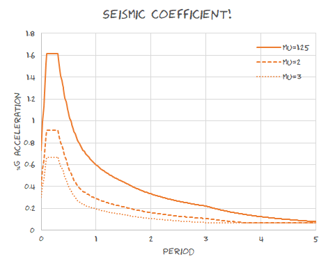
The code is outlined in Part 2. The data for the following graph of 3 series was created by four formulas in four cells. The power of VBA and a few arrays….