In this final instalment let’s use the functions. They should hopefully be self-explanatory with the VBA comments, but there are a couple of subtleties to be aware of.
The first point is that at certain time periods there are transitions between some of the governing curves. So, if plotting the spectrums over some time interval you need to make sure you have a period entry at that transition point. This is of particular importance if you are interpolating for D subsoil classes, as an abrupt transition/step occurs at 0.1 seconds. So, to plot it properly you need to have a period of 0.1 seconds and a period ever so slightly below 0.1 seconds. From the previous post we had an example of this occurring: –
Luckily for you there is a function within the file on GitHub which generates a period sequence and includes all the relevant transition points of interest and allows you to say generate this sequence between zero seconds and some other period whilst generating points at some fixed interval along the way. For the chart above the transition points or points of interest where some criteria change or start/stop to influence the calculated values are shown below for one of the spectrums: –

These points correspond to the transitions between the various spectral shape factor curves, interpolation between C & D soils points, where near fault factors start to influence the curves, etc. Some of the transition points are easy to spot, others not so much. So, use the function provided essentially.
Usage example
Let’s do an example based on designing a hospital in Wellington using the following parameters: –
| Location | Wellington, NZ |
| Hazard factor | 0.4 |
| Return period factor (IL4 structure) | 1.8 |
| Subsoil classification | D |
| Site period | 0.87 seconds |
| Distance to nearest fault | 2 km |
| Period range of interest | 0 to 5 seconds |
| Calculate coefficient at max intervals of: – | 0.015 seconds |
| Ductility | 2.0 |
| Structural performance factor | 0.7 |
| Analysis type | ESM |
Let’s start by generating the period range, this uses the Loading_generate_period_range function: –
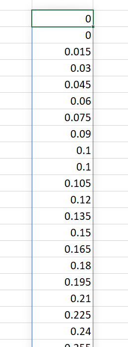
=Loading_generate_period_range(period_range_limit, period_step)For our problem, we want to generate a range of periods between zero and five seconds, at intervals of 0.015 seconds: –
=Loading_generate_period_range(5, 0.015)If we enter this in a cell, we get a dynamic range created with our period sequence, consider this sequence as being a variable T_1: –
Now to generate the sequence of seismic coefficients based on the above period we use the Loading_C_d_T function: –
=Loading_C_d_T(T_1, Site_subsoil_class, Hazard_factor, Return_period_factor, Fault_distance, mu, S_p, ESM_case, D_subsoil_interpolate, T_site)So, for our example we have D soils and the geotechnical investigations have reported the site period, so we would want to use the interpolation between C & D soils. We also want to undertake an Equivalent Static Method analysis. The last three parameters are optional, but in this case, we want to use them: –
=Loading_C_d_T(T_1, "D", 0.4, 1.8, 2, 2, 0.7, TRUE, TRUE, 0.87)If we enter this in a cell with T_1 referring to the range of the periods we create a sequence of seismic coefficients: –
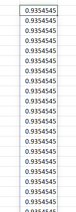
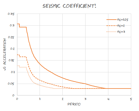
If we were to plot these on an XY scatter chart with X values being the period range and the Y values being the seismic coefficients, we get the following chart of the seismic coefficient between zero and 5 seconds for our particular site. Easy! No more interpolation! No more mistakes

Note that the Loading_C_d_T function is the only function that works with period arrays like shown above (as well as with a single cell input). The other intermediate parameters can only accept a single period value from a single cell.
Conclusion
Hopefully, this makes your life easy in future when it comes to calculating seismic coefficients in accordance with NZS1170.5.
No more interpolation! No more mistakes!
Me (2020)
Refer to the VBA code for a full description of all the functions and parameters. If in doubt leave a comment here or raise an issue on GitHub….
Part 4 covers generating an ADRS curve and can be located here.