In the last post in this series we looked at a semi-real scenario where a rational elastic buckling analysis was undertaken in which we were able to determine the axial capacity of a system of members. The exact type of system of columns is sometimes referred to as a ‘lean-on’ system, whereby the column carrying no load helps to increase the capacity of the supported column. Basically, if we make the supporting column (or in other words the bracing system for the RHS) stiff enough it has the effect of producing a higher mode of buckling in the supported RHS column.
Basically, something where it would be hard to guess the exact behaviour and hence capacity, becomes easy peasy. It would be hard to guess the exact effective length factor  (in AS4100/NZS3404 terminology) or
  (in AISC360 terminology) for anything but the simplest of scenarios.
So now that we’ve graduated with respect to axial buckling, let look at some flexural torsional buckling analyses where guessing gets a whole lot more impossible. This is where it gets a little harder, but not much harder, and once you know what you’re doing it’s guaranteed to blow your mind.
Bring on the moments…
In AS4100 or NZS3404 the design is normally you are just following the normal canned rules for determining the effective length for evaluating the capacity of a beam in bending. Easy right, so why would I need all this buckling analysis carry on when looking at bending?
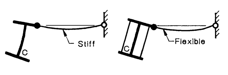
Well because often real-world situations regarding restraint conditions don’t really easily classify themselves as the perfect idealised Fixed (F), Partial (P) or Lateral (L) restraints. They often don’t idealise down to the nice pictures in the code, for example this type of thing: –
So, let’s start easy like we did with the axial case by demonstrating how it works. For this we will need Mastan2, it’s free, and free is good.
Let’s go about justifying via a flexural buckling analysis the theoretical reference buckling moment ( ) defined in CL 5.6.1.1.1(d) of NZS3404, or CL 5.6.1.1(a) of AS4100 as being the following rather daunting equation: –
![M_o= \displaystyle{ \sqrt{\bigg\{\bigg(\frac{\pi^2 EI_y}{L_{e}^2}\bigg)\bigg[GJ+\bigg(\frac{\pi^2 EI_w}{L_{e}^2}\bigg) \bigg] \bigg\} }}](https://engineervsheep.com/wp-content/ql-cache/quicklatex.com-54588ea2459b1310a5f5b191f493852d_l3.png "Rendered by QuickLaTeX.com")
Before we get into it, what exactly does this equation represent, well it’s the theoretical buckling moment for a beam loaded with a uniform moment gradient with twist restraints at supports. This means a constant bending moment over the full length, corresponding to the  condition. Now in reality not many beams are loaded with constant bending moment, this is where the
  factor comes in (similar concept the the
  factor in AISC360). This basically scales up or down the theoretical reference buckling moment so that we can apply it to other moment distributions.

 reference moment distribution
Why do we do this, well because the equation above can be derived from first principles for a constant moment case (according to textbooks, your lecturer, apparently easily…). Anything else and shit gets too hard to do it by hand, so we give up and come up with a means of fudging it all to give the right answer via a scaling factor that is dependent on the shape of the moment diagram. The exact mechanics are not important, what is important is that it works.
Now, an important thing to appreciate here is that the reference buckling moment is not a design capacity. More on this later on when we introduce the  factor. But let’s walk before we run!
So lets prove it works, firstly lets setup a model with a constant moment case and check the same thing by hand using the equation above and via a buckling analysis.
Reference buckling moment via equation:-
Let’s say we have a 410UB54 beam thats 8m long, for the case we have this means the effective length ( ) is 8m long: –
Therefore, for a 410UB54, we have the following section properties: –


Note that mastan2 takes  so we are doing the same here for consistency even if
  is the generally accepted value in NZS3404 for the Shear Modulus, where
  for steel


With  :-
:-
![M_o= \displaystyle{ \sqrt{\bigg\{\bigg(\frac{\pi^2\times205000\times 10.3\times10^6 }{8000^2}\bigg)\bigg[78846.15\times234\times10^3 +\bigg(\frac{\pi^2\times205000\times 394\times10^9 }{8000^2}\bigg) \bigg] \bigg\} }}](https://engineervsheep.com/wp-content/ql-cache/quicklatex.com-164f6a5c1dbfef918db46d87d5d816d5_l3.png "Rendered by QuickLaTeX.com")

Reference buckling moment via buckling analysis:-
Firstly, let me say Mastan2 is unitless, so ensure you work in consistent units for consistent answers.
Our mastan model with  equal and opposite moments applied at each end. Beam has twist restraint at ends, the equivalent of a ‘F’ restraint. Note that beam is divided into at least 8 segments, so we get accurate buckling moments, warping is also set to continuous (this is quite important, don’t be that guy who forgets this!).
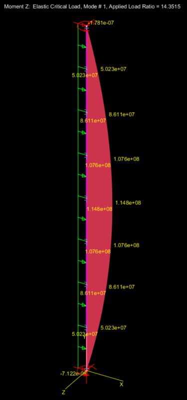
Run an Elastic Critical Load analysis and display the moment: –
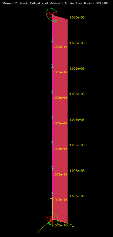
Now you’ll note at the top the applied load ratio (and maximum applied moment) is  , this is equal to
  . Since this is the reference case the Applied Load Ratio = basically.
Now you will note therefore based on our elastic buckling analysis that  . Noting of course we have perfect agreement (thankfully).
Some other similar checks to enhance the amazing things you just learned…
Lets test for a second case, namely one of the known cases for which a known (possibly) analytical solution exists, namely those outlined in table 5.6.1 of NZS3404.
Based on what I’ve told you previously, the critical buckling moment (by this we mean the maximum moment sustained) from our buckling analysis should be equal to right? well let’s see if we get this result.
Randomly choosing this case, lets calculate for point loads at the 3/8 and 5/8 span locations: –
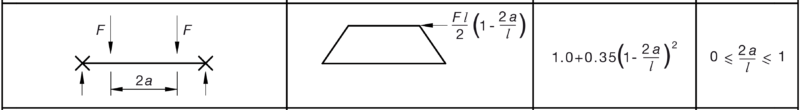

Therefore 
So in theory our elastic buckling load from the buckling analysis should equal  if the equation for is actually correct. It’s probably a bit of an estimation in terms of curve fitting, but let’s see how we go as you’d expect it to be fairly close.
Lets add some point loads symmetrically about the centreline and run that Elastic critical load analysis again:-
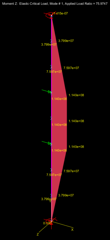
You’ll note the maximum moment is  , not quite the
  predicted. So in effect from the buckling analysis
  . This is basically what CL 5.6.4 is saying, though it’s written in a confusing way (to me at least).
While not in complete agreement, we don’t actually know if the equation is based on a curve fitting exercise. We can see though if you used the equation you’re a little unconservative compared with the true theoretical result.
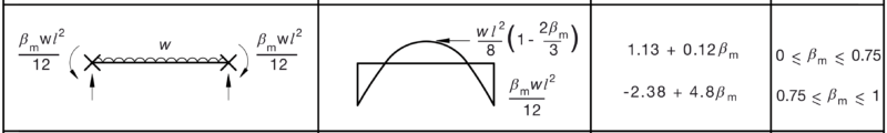
It might be interesting here to calculate using the following equation which is given as an option in the code:-


Again higher than both the equation from Table 5.6.1 & the buckling analysis.
Third times a charm… to rub it in
Now, let’s test a third case, the simply supported case with a UDL, we should get  if we believe the equation presented below: –
Mastan2 result:-
You’ll note the maximum moment is  . So in effect from the buckling analysis
  . Pretty good agreement I think.
Conclusion
So to recap, you can use a buckling analysis to determine the reference buckling moment and . Both of which you need to know to calculate a design capacity.
As you can hopefully appreciate, while we are looking at fairly simple cases here, the technique extends to any type of situation imaginable, be it restraints or moment distribution.
While we have this equation for the case of any moment distribution: –
It is just an estimate based on curve fitting, the buckling analysis route allows you to get the theoretical buckling moment and moment modification factor directly. Ka–f-ing–boom….. blew your feeble mind with the infinite possibilities that exist now before you now that you know this?
Now I want to stress here, these moments coming out of the analysis are NOT the design capacity, you need to still apply the factor and a strength reduction factor to get to a design capacity. This is similar in a way to how we had to apply the  factor for the axial buckling checks in previous posts, taking a theoretical buckling load to a design buckling load. Basically the factor accounts for things like any initial imperfections, residual stresses, 2nd order effects. Ensuring (hopefully) a lower bound capacity is calculated for design purposes.
Part 4 here.
Great series of posts! I also find CL 5.6.4 of AS 4100 very confusing. In particular CL 5.6.4 b) which advises that the moment magnification factor is to be calculated as Mos/Moo which I do not understand.
Thanks for the comment!
I’ll do another post demonstrating my own interpretation of what this particular sub-clause means. I seem to get answers for alpha_m using this approach that are very similar (usually a little higher) than using the values out of the tables or the equation that uses the quarter & half point moments. But it’s a lot of additional work and not that practical except for the smallest of buckling analyses.
EDIT – check out part 6 here
That was how I learnt and understood Mo – the steel beam capacity is a function of Mo and the bending moment diagram shape. Buried in there somewhere is the critical buckling flange of the beam. Good work and explanation.
Can the beam be a nice brown colour?