Part 6 – Slicing & Dicing
Based on the last two posts, I’d now reached the stage where I’d determined the general basis for calculating the force and centroid of the concrete compression force. This seemed like one of the major challenges had been overcome, just a matter of coding it now I guess.
Going Off Script…
However for a moment I’d like to touch on the inherent errors in other approaches, because you’re probably thinking all this integration is a bit over the top at the end of the day. When you’ve done these things before, you just obliviously divided the compression region up into some discrete strips and were none the wiser. It’s probably close enough after all considering all the other inherent variability in material properties, time is money man.
Other software I’d come across seemed to take the route of modelling the stress/strain relationship as a series of discrete values connected by linearly interpolated values. For the EC2 parabolic curve they seemed to simply estimated the centroid as some crude average in the middle of the compression area in the worst cases or actually calculated the centroid of the resulting 3D wedge like shape of stress in the best cases. But obviously due to the assumptions around estimating the parabolic part of the stress curve as a series of discrete points connected by straight lines, this approach starts to introduce some level of error.
Provided the steps/divisions are small enough I guess this approach can get you close enough to the true value. But in reality are you actually dividing it into 1000/10000/100000 equally spaced divisions? Somehow I don’t think so, and that’s the thing, unless you work something out exactly to compare, how do you know how close you really are to the true mathematical answer. What error you are inherently accepting?
The general population of sheep might be happy with this approach, but I needed to satisfy and channel my inner engineers OCD here. My gut told me if taking this approach I’d need to divide the section into a ridiculous number of slices which would become quite computationally expensive if I was after any sort of accuracy.
I must confess I initially also started down this route of using linear interpolation of the true curve, drawing 1001 little wedge shaped regions of stress in an effort to find out what the volume was, and where the centroid was. I was in danger of being one of those damn sheep unless there was an intervention!
At some point I stood back and asked what the hell am I doing, my inner OCD demons got the better of me and self corrected the poor life choice I was attempting to embark on. Being made aware of the inherent errors in this approach especially at a relatively crude number of divisions, it seemed there was only one way to satisfy those demons. Bloody integration and working based on first principles is the answer to everything it seems. Perhaps my high school math teachers were right after all, calculus was going to be useful… F-ing demons, you better be right as I take the metaphorical red pill, diving into what I perceived to be the harder route at that point in time.
Back on Script…
At least the beauty of the way I am doing it as I see it at least, is that there is no error involved and I can as a result actually live with myself. It’s the exact answer within whatever tolerance you accept with respect to the numerical integration and other iterative solvers techniques being used. Machine precision if you so desire or at least a sufficient number of decimal places to please anyone.
Back in reality, depending on the shape of the section and the resulting compression area. I knew I’d have to calculate the force and centroid parameters for quite a few smaller subregions in each individual horizontal slice.
Basically the idea was to slice the section horizontally at points of interest and find all the forces/centroids for all the resulting triangular and trapezoidal regions that are formed. Then its a simple calculation to find the overall force and resulting centroid location of the resultant concrete force. Then at that point we have basically completed the concrete force portion of the analysis (apart from repeating the process as many times as it takes to iteratively solve for overall equilibrium for any given configuration of section, reinforcement and axial load).
An issue with doing all the required geometrical transformations, rotations, intersections, etc is that you sometimes hit the limitations of the precision your tool of choice uses. Due to the inherent approximation of numbers like taking the sin/cos of an angle, you can get into the situation where you might rotate some geometry by 30 degrees, and then alternatively rotate the same geometry by two successive lots of 15 degrees and the resulting x & y coordinates don’t quite agree to some arbitrary level of precision.
For example your computer as I understand it, uses Taylor series approximations to estimate trigonometric operations. So these operations are subject to rounding and machine precision issues just like anything else. 1.0000000000000 can turn into 0.99999999999998 pretty quick. Excel is pretty terrible at this as it only essentially has 15 significant figure precision, add two numbers together that differ by a large order of magnitude and you’ll see what I mean, numerical accuracy is not Excels strong point.
Apparently Python works internally to 53 bits of binary precision, called double precision. Which is obviously much better than Excels arbitrary 15 significant digits it retains for use in calculations. But this means every number is essentially an approximation if you drill down to enough significant figures. Working with floats in Python can produce some mathematical weirdness when rounding for example due to the approximate nature of the numbers, numbers you expect to round down round up and so forth. A demo to show this perhaps:-
>>> from decimal import Decimal
>>> Decimal(2.675)
Decimal('2.67499999999999982236431605997495353221893310546875')
# this is the true approximation for 2.675

>>> round(2.675, 2)
2.67
# see how in this scenario 2.675 was rounded down instead of the expected answer of 2.68 because the approximation for 2.675 is actually slightly less than 2.675
I’m mentioning it because for certain operations I was relying on I came up against this very issue. Looking up a float value in a list or array to try find it’s index is one example of what might fail. Because due to machine precision or limitations in some of the algorithms, the number you are looking for is ever so slightly different due to the inherent approximations noted above so there is no match.
To get around this you just have to get creative and do things slightly differently to work around these types of things occurring and throwing a virtual spanner into your code.
While we are off topic again, I’d also mention at this point that planning what you are trying to achieve is always a good thing. Think logically, it’s what differentiates an ordinary engineer from a good engineer when it comes to certain things. I often fall into the trap of coding rather blindly, fudging and bodging until it works, then I try my best to optimise the code further without breaking the functionality I’ve created. Often I look back and think I should have had a better plan and I might have avoided that error that wasted half a day of my life tracking down, or start out using more efficient means of doing things from the start, or simply would have gone about it in a different way in hindsight. I probably didn’t do enough planning in hindsight, so if there’s a better way of doing things I’m all ears.
Why you are really here after all…
Pretty pictures, right? Enough of the slightly off topic ramblings.
The following images and code snippets illustrate the general logic, so rather than discussing it to the nth degree a few pictures explain things a lot better than a few thousand words.
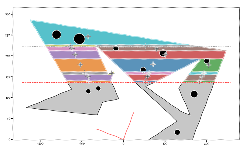
Basically stepping through each section slice, determining the individual regions in each slice, then calculating the force and centroid is what we are showing here:-

# geometry object for this slice is:-
MULTIPOLYGON (((1.256863804268402 162.057569492655, -32.3832904842091 193.210231132028, 186.2556460172985 193.210231132028, 124.3862680697111 162.057569492655, 1.256863804268402 162.057569492655)), ((-53.69202197667455 193.210231132028, -39.82196339111482 162.057569492655, -149.6921415307834 162.057569492655, -168.411487113557 193.210231132028, -53.69202197667455 193.210231132028)), ((239.8128956991505 193.210231132028, 227.8545093001678 162.057569492655, 162.4466479382758 162.057569492655, 186.2556460172989 193.210231132028, 239.8128956991505 193.210231132028)))
# as you can see, this slice is made up of 1 MultiPolygon object consisting of 3 Polygon objects, calculated centroids shown with the target marker
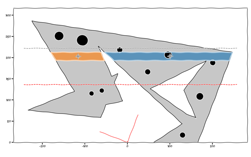
# geometry object for this slice is:-
MULTIPOLYGON (((-32.3832904842091 193.210231132028, -53.35915236560266 212.635050714651, 247.2693853239711 212.635050714651, 239.8128956991505 193.210231132028, 186.2556460172989 193.210231132028, 186.2556460172992 193.2102311320284, 186.2556460172985 193.210231132028, -32.3832904842091 193.210231132028)), ((-62.34050886180128 212.635050714651, -53.69202197667455 193.210231132028, -168.411487113557 193.210231132028, -180.0836811257238 212.635050714651, -62.34050886180128 212.635050714651)))
# as you can see, this slice is made up of 1 MultiPolygon object consisting of 2 Polygon objects, calculated centroids shown with the target marker
Rinse and repeat for all slices.
Once again using the shapely package, its a fairly trivial exercise to intersect the base section geometry in the manner demonstrated above and slice things up. Depending on what’s going on in the slice, you either end up with a Polygon, a MultiPolygon, a Point, a LineString, or a GeometryCollection object containing any combination of the above objects as demonstrated above.
Then its a matter of wrapping some logic around sorting out the individual Polygon objects and discarding the Points and LineStrings. These unwanted objects occur when you get the tip of a triangular region on one of the slice lines for a Point, or when the slice line coincides with a regions edge for a LineString. All we are interested in is the Polygon objects formed by slicing up the section, as these have an area, and that’s what we are basically interested in after all.
That’s all I’ll say on that, go take a look at the source code (once its public) if you can’t contain your excitement about how marvelous all of this appears to be.
One thing I will point out is evaluating the integrals is dead easy in Python. I simply used the scipy.integrate function quad, this is based on a Gaussian Quadrature integration technique as far as I can tell. This may change once I’m all finished and looking to speed things up, but it doesn’t seem to be a limiting factor based on initial testing.
I’m not going to explain the Gaussian Quadrature technique in detail, but suffice to say I vaguely remember a lecturer in third year at university trying to teach it to us, spending a grand total of one lecture on it I think to solve some random problem. Essentially doing an exceedingly poor job of getting us to understand this new and strange integration technique.
So as it would eventuate, naturally this equates to the fact that the end of semester exam would heavily rely on some questions that would require the technique. FML, as it turns out about 2% of the students attempted this lecturers questions as they foolishly gave us a choice. Quite smart of the lecturer actually, limited their workload marking the damn thing I guess.
Long story short, turns out its kind of a cool technique once you get a handle on what it’s doing and very fast. I’ll leave you to look into it though as any explanation I have simply won’t do it justice.
Conclusion
I’m pretty chuffed with myself at this point, but its not over until I’ve gone and implemented some way of solving the whole equilibrium thing so we can spit out some moment capacities. Then doing that a few thousand times or so to create an actual interaction diagram.