Following on from the previous blog posts in this series that provided functions for calculating the NZS1170.5 seismic coefficient. I’ve added some further functions to the GitHub repository that utilise the previous functions to generate an ADRS curve in accordance with the provisions of NZS1170.5 and the draft Seismic Assessment of Existing Buildings guidelines produced by MBIE in NZ.
What is an ADRS curve you might ask, well it’s an Acceleration Displacement Response Spectrum, and they look like the below image (the pink line) if you’ve generated them correctly (fingers crossed). While at first glance it looks suspiciously like the “normal” period vs acceleration plot, don’t be fooled!
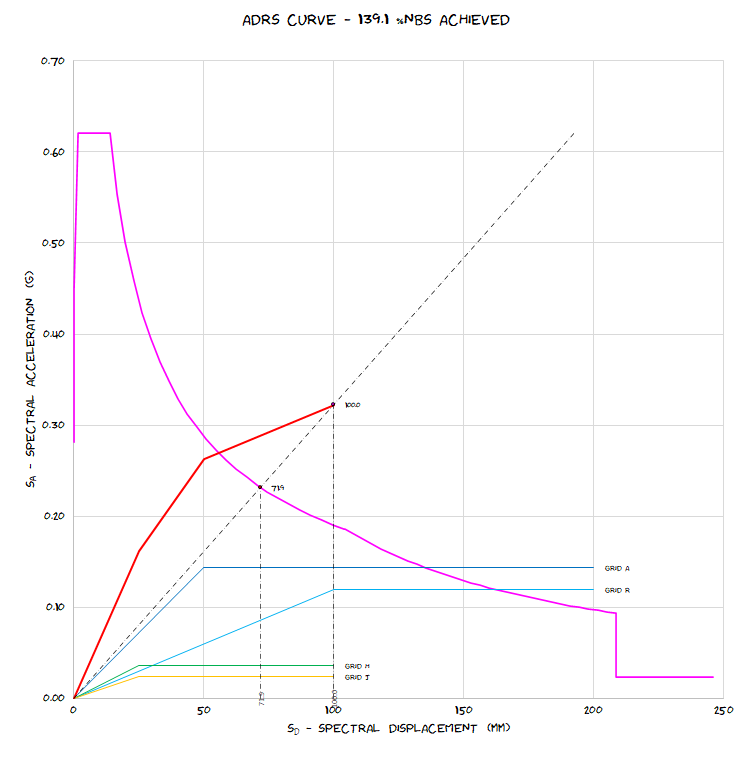
It’s essentially another way of visualising the design response spectrum, but in terms of displacement and acceleration.
Usually the “normal” response spectrum is plotted in terms of period on the horizontal axis, and acceleration on the vertical axis. The ADRS curve is simply plotting the same thing after some conversions but as a displacement on the horizontal axis, and acceleration on the vertical axis.
A straight line drawn from the origin to the curve represents a specific period.
This representation of the design spectrum is used in displacement-based design. In NZ when assessing existing buildings, we are “encouraged” to use a displacement-based approach. The idea being that force-based approaches don’t work too well for accurately assessing the strength and more importantly the deformation capacity available in existing structures.
What the ADRS curve allows us to do is evaluate the collective response of the bracing elements in the lateral load resisting system for a structure even if they have different ductilities and or deformation capacities, and determine the overall capacity for a structure.
This is achieved usually via the use of a simplified hand-based pushover analysis to inform the designer of the overall available deformation capacity. The particular analysis method we use in New Zealand is called SLAMA (Simple Lateral Mechanism Analysis).
Enough of the background (if you must know more, check out the guidelines I linked to above), onto the VBA code: –
The code
Function Loading_ADRS(T_1 As Variant, Site_subsoil_class As String, Hazard_factor As Double, Return_period_factor As Double, _
                      Fault_distance As Variant, S_p As Double, zeta_sys As Double, _
                      Optional D_subsoil_interpolate As Boolean = False, Optional T_site As Double = 1.5) As Variant
'function to calculate the spectral displacement and spectral acceleration for plotting an ADRS Curve (Acceleration Displacement Response Spectrum)

'________________________________________________________________________________________________________________
'USAGE
'________________________________________________________________________________________________________________
'=Loading_ADRS(T_1,Site_subsoil_class,Hazard_factor,Return_period_factor,Fault_distance,S_p,zeta_sys,D_subsoil_interpolate,T_site)
'T_1 = FIRST MODE PERIOD
'Site_subsoil_class = SITE SUBSOIL CLASS, i.e. A/B/C/D/E (ENTERED AS A STRING)
'Hazard_factor = HAZARD FACTOR Z
'Return_period_factor = RETURN PERIOD FACTOR Ru OR Rs
'Fault_distance = THE SHORTEST DISTANCE (IN kM's) FROM THE SITE TO THE NEAREST FAULT LISTED IN TABLE 3.6 OF NZS1170.5
'                 IF NOT RELEVANT USE "N/A" OR A NUMBER >= 20
'S_p = STRUCTURAL PERFORMANCE FACTOR
'zeta_sys = SYSTEM DAMPING (AS A PERCENTAGE)
'OPTIONAL - D_subsoil_interpolation is optional - TRUE/FALSE - consider interpolation for class D soils
'OPTIONAL - T_site is optional - Site period when required for considering interpolation for class D soils
'           (note default value of 1.5 seconds equates to no interpolation)
'________________________________________________________________________________________________________________

    Dim results As Variant
    Dim C_d_T As Variant
    Dim K_zeta As Double
    Dim i

    'determine the spectral damping reduction factor
    K_zeta = Loading_K_zeta(zeta_sys)

    'determine the 5% damping Response Spectrum design spectrum with ductility of 1.0 (so k_mu = 1.0)
    C_d_T = Loading_C_d_T(T_1, Site_subsoil_class, Hazard_factor, Return_period_factor, Fault_distance, 1, S_p, False, D_subsoil_interpolate, T_site)

    ReDim results(LBound(T_1) To UBound(T_1), 1 To 2)

    For i = LBound(T_1) To UBound(T_1)

        'determine the spectral acceleration (S_a)
        results(i, 2) = K_zeta * C_d_T(i, 1)
        'determine the spectral displacement (S_d)
        results(i, 1) = Loading_K_delta_T(T_1(i, 1)) * results(i, 2)

    Next i

    'return results
    Loading_ADRS = results

End Function

Function Loading_K_delta_T(T_1 As Variant) As Variant
'function to calculate the Displacement spectral scaling factor

'________________________________________________________________________________________________________________
'USAGE
'________________________________________________________________________________________________________________
'=Loading_K_delta_T(T_1)
'T_1 = FIRST MODE PERIOD
'________________________________________________________________________________________________________________

    Dim pi As Double
    pi = 3.14159265358979

    Loading_K_delta_T = 9810 * T_1 ^ 2 / (4 * pi ^ 2)

End Function

Function Loading_K_zeta(zeta_sys As Double)
'function to calculate the spectral damping reduction factor

'________________________________________________________________________________________________________________
'USAGE
'________________________________________________________________________________________________________________
'=Loading_K_zeta(zeta_sys)
'zeta_sys = SYSTEM DAMPING (AS A PERCENTAGE)
'________________________________________________________________________________________________________________

    Loading_K_zeta = (7 / (2 + zeta_sys)) ^ 0.5

End Function
Usage example
Let’s create the ADRS curve for the same Welington site we had in the example in part 3.
| Location | Wellington, NZ |
| Hazard factor | 0.4 |
| Return period factor (IL4 structure) | 1.8 |
| Subsoil classification | D |
| Site period | 0.87 seconds |
| Distance to nearest fault | 2 km |
| Ductility | 2.0 |
| Structural performance factor | 0.7 |
Firstly, we would generate our period range in the same manner as we did in part 3 using the Loading_generate_period_range function, so we won’t cover that here again. As noted in part 3, it’s important to use a period range if plotting the curve that accounts for all the transition points between all the various factors.
Next, we need to know the equivalent viscous damping of the system, this scales the spectrum to account for ductility. If our curve is going to be in accordance with the Seismic Assessment of Existing Buildings guidelines, then we can use appendix C2D in section 2 of the guidelines to determine this.
Let’s say for the sake of the example that our structure was a Reinforced Concrete (RC) frame, then we can assess the system damping to be 5% inherent damping + 10% hysteretic damping for a system ductility of 2.0. Therefore, the total equivalent viscous damping of the system = 5 + 10 = 15%.

To generate our curve assuming our range of periods is in a sequence referred to as being a variable T_1: –
=Loading_ADRS(T_1, Site_subsoil_class, Hazard_factor, Return_period_factor, Fault_distance, S_p, zeta_sys, D_subsoil_interpolate, T_site)For our particular problem we would enter the following in a cell to generate the ADRS curve coordinates. It’s worth noting here that the ADRS curve requires the use of the Response Spectrum derived spectral shape factors.
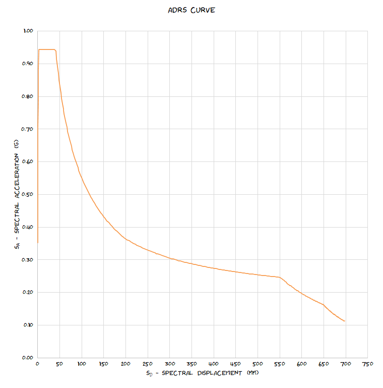
=Loading_ADRS(T_1, "D", 0.4, 1.8, 2, 0.7, 15, TRUE, 0.87)If we enter this in a cell with T_1 referring to the range of the periods we get the following result: –

The blue column (1st column of the functions results) is the spectral displacement and the red column (2nd column of the functions results) is the spectral acceleration: –
Plot these on an XY scatter chart and you get the final ADRS curve: –
Now that we have our ADRS curve, we can show that for any points we plot that it describes the stiffness (or in other words the period).
The stiffness of a structure can be represented by radiating lines from the origin
of the acceleration-displacement response spectrum. These lines, for periods with 0.5 second increments are plotted on the same curve below to show the concept: –

Code Update…
Note I’ve made a few small tweaks to the code on GitHub to address some inconsistencies I noted while writing this post. Part 2 has been updated, so if you downloaded the code from GitHub previously, make sure you download an updated version.
Part 5 can be found here, explores how to get the functions working in non-Excel 365 versions of Excel.
Hi, firstly, this is an incredible blog – thank you a lot. I have a question, however, can the functions only be used in excel 365 as opposed to 2019? I am getting a #NAME error when i try run it.
Cheers
Hi Jason,
I don’t see why they wouldn’t work in excel 2019, but there maybe something I’m not aware of.
You grabbed the module from github, and imported it into it’s own module vs copying all the individual functions into a sheet module (in case something was missed)?
A #NAME error in excel suggests you’re not even seeing the function in the workbook, potentially putting it into a sheet module and trying to call the function from another sheet could do this as well? Make sure the functions are not in a sheet, but instead in a separate module. Importing the functions from the ‘bas’ file on GitHub should do this.
Let me know if you still have issues and I can share an example file with it setup to see if you see the same issue.
Hi Jason, going through the code, I believe the worksheet function SORT is only available in excel 365. I used this in function https://github.com/Agent6-6-6/NZS1170.5-Seismic-Coefficient-functions/blob/6dcb19f81434274350273486608e15976169bb11/NZS1170_Seismic_Coefficient.bas#L586
I can update with an alternative means of sorting so it will work on excel 2019. Give me a few days.
Hi Jason
I’ve updated the code to add an alternative sorting algorithm, which should (fingers crossed) make it work in Excel 2019. Please test and let me know if you have any further problems.
You can download the latest NZS1170_Seismic_Coefficient.bas module from the following link:-
https://github.com/Agent6-6-6/NZS1170.5-Seismic-Coefficient-functions
Hi,
Unfortunately it’s still not working. I am getting a #VALUE error now though. I have a feeling that 2019 doesn’t support dynamic arrays/spilled cells. Let me know your thoughts. Thanks
Yeah possibly that’s an issue, had not thought of that.
You can still generate your own period range on a sheet, (like 0, 0.1, 0.2, etc) and use the ADRS function on a single period cell instead of the entire period range. Then drag down to cover all period inputs. That should work?
Hm thats not working as well. I downloaded a trial version of 365 and its working fine. I think I might just develop a spreadsheet using that and then when the subscription expires, use 2019 – should work hopefully.
I wonder if it will work by entering as an array formula (instead of pressing enter when entering the formula, try shift+ctrl+enter?)
Nope didn’t work either unfortunately
IS 2 the prefomrance factor or the ductility and what is true and false for the soil D
Sorry I don’t understand the question related to ‘is 2 the preformance factor or ductility’.
For D subsoil type, depending on the site period the NZS1170.5 code allows interpolation between C and D soil types. Refer to NZS1170.5 for details.